Advent Day 20: Pixels and classification
Dec 20, 2025
Maps often feel intuitive. Forest here, grassland there. High NDVI in green, low in brown. Beneath these clean visuals lie two layers of abstraction that shape how we interpret patterns: pixels and the classifications applied to them. Understanding both is essential, because misleading results arise from how continuous variation is captured in pixels and translated into discrete maps.
A pixel is the fundamental unit of a remote sensing image. A pixel is a square representing an area on the ground for which a single set of values is recorded across spectral bands. A pixel is not an object, it does not correspond to a tree, a patch of grass, or a habitat type. It integrates all surfaces and structures within its footprint and is influenced by its surroundings. When landscapes are heterogeneous, a single pixel may capture multiple surfaces. These so-called mixed pixels are unavoidable, especially at coarser resolutions. Pixels reduces complexity into something visually tidy, rather than faithful to reality.
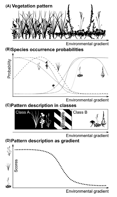
Classification is the next step; classification is the process that transforms pixels into classes to make maps. All classification approaches impose structure. They decide which differences matter, where boundaries are drawn and how ambiguity is handled. These choices shape the final product as much as the underlying data. For instance, this figure from Feilhauer et al 2021 shows the different ways that vegetation patterns can be characterized with remote sensing data. This whole paper is great and worth the read, it links remote sensing concepts to ecological theories so nicely and shows how analytical choices with remote sensing data can embed ecological assumptions (and if you want a deep dive on this topic check out co-author Giles M Foody’s publications too).
Common classification distinctions include:
- Pixel-based versus object-based: Pixel-based methods classify each pixel independently using spectral information alone. Object-based methods first group neighboring pixels into spatial units representing actual objects (like a tree or a building), then classify those objects using spectral, shape, texture and contextual information.
- Supervised versus unsupervised: Supervised classification uses analyst-defined training data to assign classes, while unsupervised classification identifies patterns in the data that are interpreted afterward.
- Hard versus soft classifiers: Hard classification assigns a single class to each pixel or object. Soft approaches relax this constraint; for instance, spectral unmixing estimates fractional composition while fuzzy classification allows partial membership across classes.
Both pixels and classes distort information in important ways. Pixels average over fine-scale variation, and classes introduce artificial boundaries into systems that are fundamentally continuous. A gradual moisture gradient becomes an abrupt edge, a disturbance legacy becomes a clean category. Even smooth, continuous products are not immune with vegetation indices like NDVI being known to saturate in dense or highly productive systems, giving ecosystems the appearance of stability despite differences. These artifacts can propagate into downstream analyses, influencing estimates of habitat availability, fragmentation, or change in ways that reflect mapping conventions more than ecological reality.
Remote sensing data and products are powerful, but they are not neutral mirrors of nature. For ecologists, knowing what questions to ask before building or applying a map is as important as interpreting the patterns the derived maps ultimately display. Critically understanding remote sensing derived products begins before a map is ever made or used. Ecologists should ask how pixels are defined, grouped or mixed, how classes are trained, constrained or simplified, and which assumptions or thresholds are embedded in those choices. What ecological variation is being averaged away, and which processes become invisible at this resolution or representation? These decisions shape the map as much as the data themselves.
–
References
Feilhauer, H., Zlinszky, A., Kania, A., Foody, G. M., Doktor, D., Lausch, A., Schmidtlein, S., He, K., & Disney, M. (2021). Let your maps be fuzzy!—Class probabilities and floristic gradients as alternatives to crisp mapping for remote sensing of vegetation. Remote Sensing in Ecology and Conservation, 7(2), 292–305. https://doi.org/10.1002/rse2.188